Seventh Week: Observation 3

Dear Readers,

Today, I collected data on colors, shapes, speckles, and the weights of four largest leaves from each plants.

One concern was raised by professor Michaels that the plants from Morton's Mix are having tip burning from lack of calcium since they cannot absorb it fast enough.

Also, two plants from Morton's Mix, one plant from Freedom's Mix were diseased and two plants from Morton's Mix were dead already. However, all of the roots looked pretty healthy. (Professor Michaels called this bridging.)

Sixth Week: Data and Observation 2

Dear readers,

Today, I took some data on the length of the longest axis (mm) of the leaves and the length of the complementary axis (mm) of the leaves, so that I can measure (by a ruler) physical growth of the leaves.

Besides physical growth, I also measured the weight of two largest leaves (in grams) by harvesting (with scissors) two leaves from each plant. 

For fitting the regression line, I took the average of the weights of two leaves. I wanted to know whether there is correlation between the weight of the two largest leaves and length of the axis.

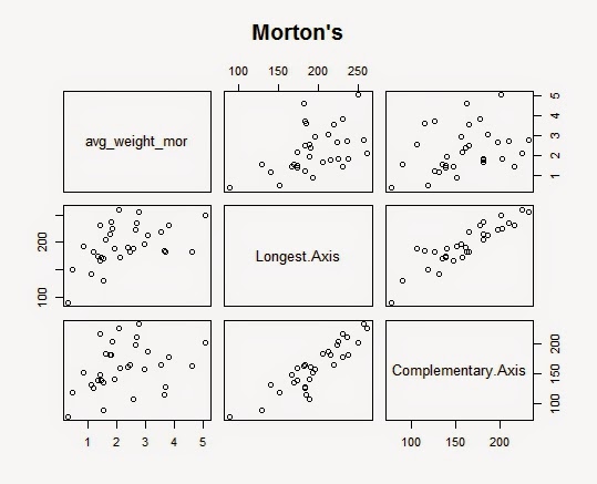
In Morton's Mix, we see a very strong correlation between the weight and the longest axis and also between the two axises. However, a relationship between the weight and the complementary axis looks mild. So, let's check the summary table for regression line of Morton's Mix.

> summary(mmod)

Call:
glm(formula = avg_weight_mor ~ Longest.Axis + Complementary.Axis, 
    data = mor)

Deviance Residuals: 
    Min       1Q   Median       3Q      Max  
-1.4458  -0.5931  -0.1255   0.6400   2.8105  

Coefficients:
                   Estimate Std. Error t value Pr(>|t|)   
(Intercept)        -0.92087    0.95130  -0.968   0.3410   
Longest.Axis        0.02926    0.01047   2.795   0.0091 **
Complementary.Axis -0.01586    0.01023  -1.551   0.1317   
---
Signif. codes:  0 ‘***’ 0.001 ‘**’ 0.01 ‘*’ 0.05 ‘.’ 0.1 ‘ ’ 1

(Dispersion parameter for gaussian family taken to be 0.9603569)

    Null deviance: 39.636  on 31  degrees of freedom
Residual deviance: 27.850  on 29  degrees of freedom
AIC: 94.368

Number of Fisher Scoring iterations: 2

From this we can see that complementary axis does not fit well in this regression line, since the p-value for the hypothesis test (null: Beta3=0, alternative: Beta3 does not equal 0) is greater than the alpha level (0.05). 

However, as I mentioned above, it might be possible to see a correlation between the two axises. So, let's try to fit a regression line for them.

> summary(mmod.2)

Call:
glm(formula = Longest.Axis ~ Complementary.Axis, data = mor)

Deviance Residuals: 
    Min       1Q   Median       3Q      Max  
-33.709   -8.752   -3.709   12.502   39.974  

Coefficients:
                   Estimate Std. Error t value Pr(>|t|)    
(Intercept)        55.61310   13.12115   4.238 0.000198 ***
Complementary.Axis  0.87302    0.07999  10.914 5.74e-12 ***
---
Signif. codes:  0 ‘***’ 0.001 ‘**’ 0.01 ‘*’ 0.05 ‘.’ 0.1 ‘ ’ 1

(Dispersion parameter for gaussian family taken to be 292.1042)

    Null deviance: 43557.0  on 31  degrees of freedom
Residual deviance:  8763.1  on 30  degrees of freedom
AIC: 276.41

Number of Fisher Scoring iterations: 2

Here, the result is as we expected. So, instead of treating the two axises as separate variables, let's combine the two and take a mean of it.

> summary(mmod2)

Call:
glm(formula = avg_weight_mor ~ avg_axis_mor, data = mor)

Deviance Residuals: 
    Min       1Q   Median       3Q      Max  
-1.4144  -0.7500  -0.2386   0.5838   2.4391  

Coefficients:
              Estimate Std. Error t value Pr(>|t|)  
(Intercept)  -0.024277   0.919078  -0.026   0.9791  
avg_axis_mor  0.012842   0.005078   2.529   0.0169 *
---
Signif. codes:  0 ‘***’ 0.001 ‘**’ 0.01 ‘*’ 0.05 ‘.’ 0.1 ‘ ’ 1

(Dispersion parameter for gaussian family taken to be 1.089074)

    Null deviance: 39.636  on 31  degrees of freedom
Residual deviance: 32.672  on 30  degrees of freedom
AIC: 97.477

Number of Fisher Scoring iterations: 2
 

Here, we can clearly see that the weight of the leaves and the axises are correlated and now the variable for axises fits the data well.

 Now, let's look at Freedom's Mix.

Here, it looks like all three variables are correlated.

 
> summary(fmod)

Call:
glm(formula = avg_weight_free ~ Longest.Axis + Complementary.Axis, 
    data = free)

Deviance Residuals: 
    Min       1Q   Median       3Q      Max  
-0.8606  -0.4031  -0.1565   0.3417   1.3652  

Coefficients:
                    Estimate Std. Error t value Pr(>|t|)   
(Intercept)        -1.328302   0.683507  -1.943  0.06173 . 
Longest.Axis        0.015163   0.004990   3.039  0.00499 **
Complementary.Axis  0.002875   0.003717   0.773  0.44551   
---
Signif. codes:  0 ‘***’ 0.001 ‘**’ 0.01 ‘*’ 0.05 ‘.’ 0.1 ‘ ’ 1

(Dispersion parameter for gaussian family taken to be 0.3716524)

    Null deviance: 21.566  on 31  degrees of freedom
Residual deviance: 10.778  on 29  degrees of freedom
AIC: 63.989

Number of Fisher Scoring iterations: 2

However, we can see that the complementary axis does not fit the data well according to the p-value shown above.

So, let's combine the two axises again and take the mean of it.

> summary(fmod2)

Call:
glm(formula = avg_weight_free ~ avg_axis_free, data = free)

Deviance Residuals: 
    Min       1Q   Median       3Q      Max  
-0.8537  -0.4079  -0.1950   0.2780   1.2990  

Coefficients:
               Estimate Std. Error t value Pr(>|t|)    
(Intercept)   -0.715077   0.561917  -1.273    0.213    
avg_axis_free  0.015976   0.003155   5.064 1.95e-05 ***
---
Signif. codes:  0 ‘***’ 0.001 ‘**’ 0.01 ‘*’ 0.05 ‘.’ 0.1 ‘ ’ 1

(Dispersion parameter for gaussian family taken to be 0.3875975)

    Null deviance: 21.566  on 31  degrees of freedom
Residual deviance: 11.628  on 30  degrees of freedom
AIC: 64.418

Number of Fisher Scoring iterations: 2

As we expected, now the axises fit the data well.

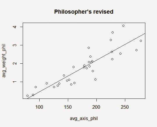
Now, let's look at the plot for Philosopher's Mix.

Here again, it seems like all three variables are strongly correlated to each other.

 
> summary(pmod)

Call:
glm(formula = avg_weight_phil ~ Longest.Axis + Complementary.Axis, 
    data = phil)

Deviance Residuals: 
     Min        1Q    Median        3Q       Max  
-0.99924  -0.29086  -0.00653   0.18672   1.07923  

Coefficients:
                    Estimate Std. Error t value Pr(>|t|)    
(Intercept)        -1.611472   0.294235  -5.477 6.75e-06 ***
Longest.Axis        0.017902   0.002865   6.248 8.08e-07 ***
Complementary.Axis -0.001399   0.003081  -0.454    0.653    
---
Signif. codes:  0 ‘***’ 0.001 ‘**’ 0.01 ‘*’ 0.05 ‘.’ 0.1 ‘ ’ 1

(Dispersion parameter for gaussian family taken to be 0.17441)

    Null deviance: 30.1881  on 31  degrees of freedom
Residual deviance:  5.0579  on 29  degrees of freedom
AIC: 39.779

Number of Fisher Scoring iterations: 2

However, we again see that the complementary axis does not fit the data well. But, we know (I checked) that the two axises are correlated.

So, let's combine the two axises and take the mean of it.

> summary(pmod2)

Call:
glm(formula = avg_weight_phil ~ avg_axis_phil, data = phil)

Deviance Residuals: 
    Min       1Q   Median       3Q      Max  
-1.0221  -0.2485  -0.0054   0.1687   1.0776  

Coefficients:
               Estimate Std. Error t value Pr(>|t|)    
(Intercept)   -1.273861   0.320245  -3.978 0.000406 ***
avg_axis_phil  0.017252   0.001734   9.951 5.14e-11 ***
---
Signif. codes:  0 ‘***’ 0.001 ‘**’ 0.01 ‘*’ 0.05 ‘.’ 0.1 ‘ ’ 1

(Dispersion parameter for gaussian family taken to be 0.2339939)

    Null deviance: 30.1881  on 31  degrees of freedom
Residual deviance:  7.0198  on 30  degrees of freedom
AIC: 48.268

Number of Fisher Scoring iterations: 2
 

Now, we see that the axises fit the data well.

p.s. the root growth looks pretty good too.

Fifth Week: Data and Observation (revised)

Dear readers,

Since we are seeing vigorous root growth, we measured the number of roots as well as the length of longest roots in mm.

When you measure number of roots, please follow the instructions in the picture (drawn by professor Michaels) below.

You should be very careful not to damage the roots when you count them since they are more fragile than you think.

From the plots, we can see some kind of correlationship between the number of roots and the length of the longest roots, except for Philosopher's Mix B. 

However, we can combine all four bins from Philosopher's Mix, since they are all from the same seed lot. Also, the seeds are all selected independently and randomly.

Here, I got a better result.

Some Changes in the Design

Dear readers,

There have been some few changes in the project design due to some problems.

Professor Michaels has notices that the one of the plants at the corner of a bin had leaves that looked slightly wilted. He immediately checked the root growth assuming that this was a plant that had not yet put down roots into the nutrient solution, but this was not the case. The roots were okay then, he realized how warm the rim of the bin lid was.

He came to conclude that when bright sunlight is streaming into the greenhouse, the dark blue plastic of the bin lids is soaking up heat, and that heat is held particularly well at the corners and edges of the bin lids where there are several layers of plastic and where the plastic might be particularly thick. Plants near the corners may be subjected to warmer temperatures than plants nearer to the middle of the lids, and this might be why he was seeing some wilting.

He solved this problem by covering the lids with aluminum foil so that the sun could not heat up the blue plastic. He also added about 1 cup of water per bin because there were some plants without roots in the solution that were beginning to wilt.

Fourth Week: Some Observations

Dear readers,

Today, you do not have much things to do in the greenhouse, since we are waiting for these lettuces to grow more so that we can take appropriate data.

Generally, they are all growing well except for one. The reason for one death might be due to the fact that it did not grow roots long enough so that roots could reach into the nutrient solution in the water. Therefore, I had to replace one from extra sample. (Remember one tray that professor Michael's took with? Yes, they were planted in case we need some extra.)

Although, extra sample was bigger than the smaller ones in the same bin, it was about the same size as the bigger ones in the bin. If you also spot some dead ones in your bins, replace them with your extra samples and make sure to label them that you replaced them with extra.

Otherwise, there are not much more things to be said today. See you all soon!

Third Week:Pots into the Water!

Dear readers,

Today, you are finally gonna put all of the pots into the hydroponics environment. But, before doing so first, you need to make holes in the lids of the plastic bins. (10-gal plastic storage boxes)
*Before this project, Professor Michaels usually just made holes into white expanded polystyrene, instead of using the lids came with the plastic bins.

First, you need to ask professor Michaels to bring out an "original polystyrene template" so that you do not have to measure distance between each pot from scratch. Put the template on the lid and all you need to do is to make a small dot with a chalk in the center of each circle.

After marking all of the lids you have, you are now going to use a drill press, an old school hole maker, to make actual holes on the lids. Before doing anything else, you should make sure to put some wooden piece underneath the lid, so that you do not make any holes in the work station.

Insert a 2-inch metal bit and then, activate the machine by inserting a key on the side hole of the drill. Set and adjust the depth stop and now you are ready to make some holes. Bring the lid and make the center of metal bit falls right onto the dot you drew on the lid. Then, carefully turn on the switch button, and drill some holes by adjusting the clamp on the right. After you are done making holes on every lid, do not forget to clean up debris in your work station.

This was what we got! Now it is the time to go back to our friend, green house. 

Then, pour water into each plastic bin up to the line you see. 

Bring out some fertilizer (Jack's Hydro Feed: http://www.amazon.com/Jacks-Hydro-16-4-17-Hydroponic-Fertilizer/dp/B00IGYELSE) add 2 tbsp to each bin then, mix it well.

Here are current sprouts. Ones in the last picture have actually taken to professor Michael's own house (since he brought them to his talk on the last weekend) and the sprouts from this tray were particularly bigger than ones left in the greenhouse here. The cause for this variability might come from the fact that the sprouts in the greenhouse were getting 11 hours of light per day while the sprouts at professor's were getting 13 hours of light per day.)

If you have noticed additional growth in each net pot, thin them out until you only have one in each.

Now, put 4 net pots to four corners of each lid and close each bin with each lid. Then, add more water through the holes and do so until you see the very bottom of the net pot on each corner touches water. This way, you can make sure that the roots will touch the water.

After you are done adding more water into each bin, remove all the net pots from each corner. Gently, place each pot with sprout into each hole. (You should make sure to keep pots from the same population together.)